In this work, we use the structure of an artificial neuron by introducing a nonlinear dynamic equation into the active function. Based on this model, it is supposed to study the state of active and passive neurons. The term neural networks refers to the networks of neurons in the mammalian brain. Neurons are its main units of computation. In the brain, they a connected together in a network to process data. This can be a very complex task, and so the dynamics of neural networks in the mammalian brain in response to external stimuli can be quite complex. The inputs and outputs of each neuron change as a function of time, in the form of so-called spike chains, but the network itself also changes. We learn and improve our data processing capabilities by establishing reconnections between neurons [1–3]. The training set contains a list of input data sets along with a list of corresponding target values that encode the properties of the input data that the network needs to learn. To solve such associative problems, artificial neural networks can work well-when new data sets a governed by the same principles that gave rise to the training data [4]. 

Activate function neuron 

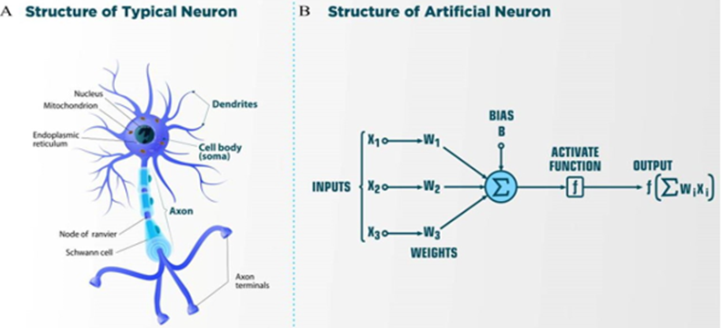
Figure.1.A. Schematic representation of a neuron. Dendrites receive input signals in the form of electrical signals through synapses. The signals are processed in the cell body of the neuron. The output signal is transmitted from the body of the nerve cell to other neurons through the axon. The Schwann cell can be in a neutral state and create a left-positive or right-negative chirality of the axon. Information is processed from left to right. On the left are dendrites that receive signals and connect to the body of the neuron, where the signal is processed. Through the axon, the output signal is sent to the dendrites of other neurons. Information is transmitted in the form of an electrical signal. Information is transmitted in the form of an electrical signal. The figure.1.B.  shows the structure of an artificial neuron. Figure.2 shows an example of the time series of the electric potential of a pyramidal neuron [5]. The time series consists of an intermittent series of electric potential jumps. Periods of rest without spikes occur when the neuron is inactive, and during periods rich in spikes, the neuron is active. Fig.2D Temporary portraits of the system (1). 

Nonlinear dynamic equation and the classical soliton model (1) for the active equation of an artificial neuron [6,7]. 

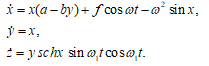
 (1)

Time portraits of the system (1) are shown in Figure.3 passive: a =1.0, b = 0.1, f = 0.02, ω = 2π, ω1 = 64π, (y0, x0, x˙0, z0) = 0.1.  Figure.4 active: a =1.0, b = 0.1, f = 0.02, ω = 2π, ω1 = 64π, (y0, x0, x˙0, z0) = 2.3.  Figure.5 active: a =1.0, b = 0.1, f = 0.02, ω = 2π, ω1 = 64π, (y0, x0, x˙0, z0) = (0.1, 2.3).   Figure.6 active: a =1.0, b = 0.1, f = 0.02, ω = 2π, ω1 = 64π, (y0, x0, x˙0, z0) = − 2.3.

The inactive states of the system are shown in Figure.5, and their inactive states are shown in Figure.2(B,C)in blue and active yellow Figure.2(A,C). Generates continuous chaotic modulation  (Figure.3 inactive (Fig.2.E.F)), violet, Figure.4,Figure.6 active ((Figure.2.E.F), green). 

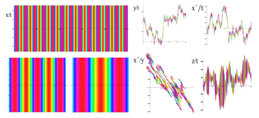
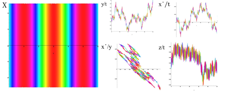
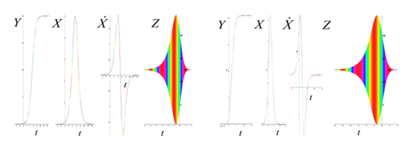
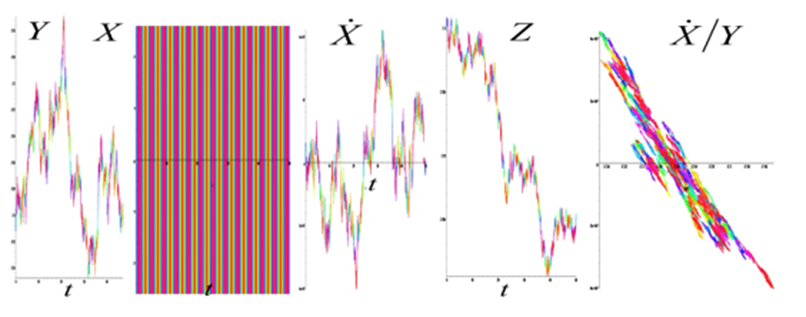
The active states of the system are shown in Figure.6, and their active states are shown in Figure.2(D) black. Generates continuous chaotic modulation (y/t, x/t, x˙/t, y/x˙). 

Artificial neural networks use a very simplified model of the fundamental computational unit, the neuron. In its simplest form, the model is simply a binary threshold unit. The network performs these calculations sequentially. Usually, discrete sequences of sample time steps are considered, t = 0,1,2,3,... Either all neurons are updated simultaneously at the same time step (synchronous update), or only one selected neuron is updated (asynchronous update). In the absence of a signal in the axon, chaotic self-excitation is observed. Mileage exists for a short time and is a stop signal. The conclusion is that this model can be used to study the behavior of a single axon.