The purpose of this study was the too early identification of Alzheimer's (AD) permits people and their health manages for medication. We have a tendency to plan an approach for classification of stages in AD and MCI, with regard to Texture with component analysis (PCA) based rule using magnetic resonance imaging (MRI) to detection of tissues in Alzheimer's Diseases. In the AD a hippocampus plays a most important affected region in the screening stage. Methods: The clinical Magnetic resonance images of brain tissue from the ADNI database having 180 AD patients, 401 MCI patients, and 200 control subjects are compared them with private OASIS dataset. The image can be stored in, jpg, bmp format and having an image size of 256x256 with the help of segmentation and SVM classification method.  For testing and performance 20 brains MRI images were used Results: For the ADNI dataset accuracy rates of up to 94% and for the OASIS brain of up to 90% were obtained.  The 91% accuracy of ADNI data is discriminated the OASIS of SVM classifiers
Conclusions: The ADNI database with PCA feature extraction is the best dataset for to classify a MRI AD Images 

Alzheimer's diseases are by a wide margin the well-known reason for dementia of maturing. As our general public ages, age-related ailments expect to expand conspicuousness as both individual and general wellbeing concerns. A clutter of cognizance is especially vital in the two respects. IN 2000, the predominance of Alzheimer's infection in the United States was assessed to be 4.5 million people, and this number has been anticipated to increment to 14 million by 2050. It centers. on Alzheimer's infection and the milder degrees of psychological weakness that may go before the clinical determination of likely Alzheimer's malady, for example, mellow intellectual debilitation [1]. It would extraordinarily profit by biomarkers that are delicate to inconspicuous cerebrum changes happening to precede the beginning of clinical side effects when the potential for the safeguarding of capacity is at the best. In vivo cerebrum imaging is a promising device for the early identification of AD through the representation of variations from the norm in mind structure, work, and histopathology [2]. It contains different biomarkers have been accounted for in ongoing writing with respect to imaging anomalies in various sorts of dementia. These biomarkers have served to fundamentally enhance early recognition and furthermore separation of different dementia disorders. In vivo mind imaging is a promising instrument for the early recognition of AD through the representation of variations from the norm in cerebrum structure, work, and histopathology [3], will be to more viable and exact finding of Alzheimer's infection (AD), and additionally, its prodromal stage (i.e., gentle intellectual weakness (MCI)), has pulled in more consideration as of late. Up until this point, numerous biomarkers have been appeared to be touchy to the finding of AD and MCI. [4]. In the meantime, the build of gentle psychological debilitation (MCI) has come to speak to a middle of the road clinical state between the intellectual changes of maturing and the most punctual highlights of Alzheimer's malady. [5] Another technique dependent on the multidimensional grouping of hippocampal shape highlights. This methodology utilizes round music (SPHARM) coefficients to show the state of the hippocampi, which are sectioned from attractive reverberation pictures (MRI) utilizing a completely programmed strategy [P8]are lead to shape investigation of hippocampi sectioned from auxiliary T1 MRI pictures on clinically analyzed dementia patients and control [6] to directly enrolled all minds to a standard layout to devise an essential shape before catch the worldwide state of the hippocampus, characterized as the point shrewd summation of all the preparation covers. We likewise included ebb and flow, slope, mean, standard deviation, and Haar channels of the shape earlier and the tissue grouped pictures as highlights [7-10] and the calculation formalizes the desire that since the precedents for preparing the classifier is pictures, the voxels, in the long run, chose for indicating the choice limit must establish spatially adjoining lumps, i.e., "areas" must be favored over separated voxels. This earlier conviction ends up being helpful for fundamentally decreasing the space of conceivable classifiers and prompts considerable advantages in speculation. [11]The kinds of the model-based methodology for thickness estimation are to naturally choose locales of intrigue (ROIs) and to successfully decrease the dimensionality of the issue [12] are utilizing a GMM which is balanced by utilizing the desired expansion (EM) calculation [13] Machine learning based arrangement calculations like help vector machines (SVMs) have indicated an incredible guarantee for transforming high dimensional neuroimaging information into clinically valuable choice criteria. In any case, following imaging based examples that contribute fundamentally to classifier choices remains an open issue. This is an issue of basic significance in imaging contemplates looking to figure out which anatomical or physiological imaging highlights add to the classifier's choice, along these lines enabling clients to fundamentally assess the discoveries of such machine learning strategies and to comprehend illness systems. The larger part of distributed places of business the subject of measurable surmising for help vector characterization utilizing change tests dependent on SVM weight vectors [14] The forget one cross-approval method is utilized to approve the outcomes acquired by the directed learning-based PC supported conclusion (CAD) framework over databases of MRI and PET pictures yielding an exactness rate up to 90.67% [15-17]

 This paper is organized follows. In section 2 the database used to test the system, pre-processing technique, filtering method with feature extraction description of methodology and classification methods used in this paper are presented. In section 3 we propose some experiments, and different results obtained with each combination are detailed.  Discussion is given in section 4 in order to analyze the experimental results obtained in this work, and the conclusions are presented in the last section.

2.1 MRI:

MRI is a non-interfering therapeutic indicative system that utilizes attractive fields in waves of radio to demonstrate body organs, tissues and so forth. It was created by Raymond Dalmatian. Be that as it may, disclosure was not inadvertent really it was slow improvement of a few creations, which was begun by Joseph Fourier, his scientific model was first utilized for attractive reverberation flag examination by Richard Ernst, at that point Raymond Dalmatian in 1974 distributed a strategy ' field centering NMR' (atomic attractive reverberation) which contained a picture of filtered volume component through a mouse [18-21].

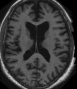
In MRI extremely solid radio waves which are multiple times more grounded than earth's attractive field are sent to a body. These radio waves propel hydrogen particle 

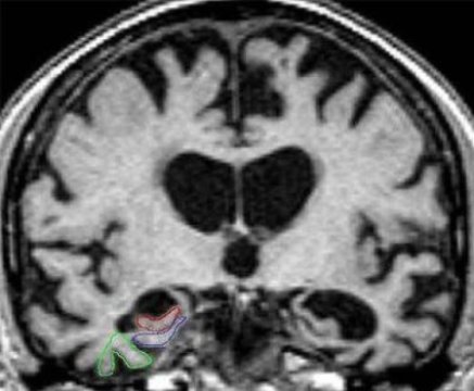
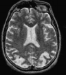
Fig 1: MRI Input Image

in the body to vibrate, and radiation which these hydrogen iotas discharge are identified outside the body and structures a picture with the help of a PC. The MRI of the human cerebrum is given in figure 1. It ignores bones as they contain little water content it for the most part fixates on fragile tissues[22]. It doesn't utilize Ionizing radiations so this procedure is moderately more secure than different systems which utilize Ionizing radiations like X-Rays. Be that as it may, for this situation, slight development can demolish the picture notwithstanding breathing can cause antiquities or picture mutilations. Differentiation medium is required for this situation which can have numerous unfavourable impacts[23-25].

2.1.1 Adni Dataset:

The information utilized in this paper was ADNI (Alzheimer's sickness Neuroimaging Initiative) database. The name ADNI was made at 2003 by the mix of three incredible national associations. The three national associations are National Institute on Aging, the national organization of biomedical imaging and bioengineering lastly the food and medications organization of some private medicinal organizations with the association[26]. The fundamental point of the ADNI to test the therapeutic pictures like MRI, PET and some natural markers, neurophysiological testing to finding an estimation of AD and MCI. To enhance the affectability of the AD to get an ideal research to create gone up against to accomplish opportune and financially savvy preliminaries[27-31]. To date, these three conventions have enlisted child more than 1500 grown-ups, ages 55– 90, to take an interest in the exploration, comprising of subjectively ordinary more established people, individuals with ahead of schedule or late MCI, and individuals with the early AD[32]. The follow-up duration of each group is specified in the protocols for ADNI-1, ADNI-2, and ADNI-GO. Subjects originally recruited for ADNI-1 and ADNI-GO had the option to be followed in ADNI-2

2.1.2ADNI MRI data:

The MRI dataset included standard T1-weighted pictures acquired with various scanner types utilizing volumetric MP-RAGE succession fluctuating in TR and TE with in-plane goals of 1.25 mm and 1.2 mm sagittal cut thickness. Just image got for utilizing 1.5 T scanners were utilized in this paper were obtained at 1.5 T MRI scanners and this database gives information to three gatherings of patients: solid patients, Alzheimer diseases patients (AD) and patients with gentle subjective manifestations (MCI). The database utilized in this work contains 1075 T1-weighted MRI images, involving 401 MCI (312 stable MCI and 86 dynamic MCI) and 188 AD. As just the main exam for every patient has been utilized in this work, 818 pictures were utilized for surveying the proposed methodology. Statistic information of patients in the database is condensed in Table 1.

Table 1: The ADNI database of the patient:

2.2 Oasis Dataset

Initially, OASIS images are related to estimates fill in as informational indexes for proceeded logical investigation. The dataset which is being utilized in this undertaking is acquired from OASIS (Open Access Series of Imaging Studies) which transparently gives the dataset containing cross-sectional MRI examines for insane and non-psychotic people going from 18 years to 96 years. The dataset comprises of 416 subjects which all are correctly given and MRI information is institutionalized T1-weighted normal from which 100 subjects have mellowed to direct dementia and 198 subjects which are everywhere throughout the age of 60.

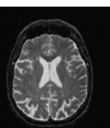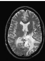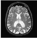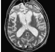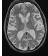MRI1	MRI2	MRI3	MRI4	MRI5	MRI6
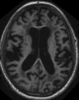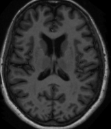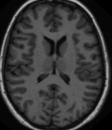MRI 7	MRI 8	MRI 9	MRI 10	MRI 11	MRI2

Fig: 2 MRI data of image feature extracted

2.3.1 PCA and texture features

The PCA is a minimal complex of pathological multivariate tests based on one vector. Its assurance can continually be probably considered to reveal the inner structure of the data in a way that best clearly explains the variance in the data. If a multivariate dataset is envisaged as a course of action of headings in a high-dimensional data space (1 rotation for each factor), PCA can provide the customer with a lower-dimensional image, a projection or " shadow " of this dissent when viewed from its most instructive point of view (in some sense; see below). This is done by only using the underlying few basic fragments with the aim of reducing the dimensionality of the changed data. PCA is strongly related to factor checking. The factor examination routinely combines more region - specific assumptions about the basic structure and handles the own vectors of an extraordinary system to some extent.

PCA is likewise identified with accepted relationship examination (CCA). CCA characterizes arrange frameworks that ideally depict the cross-covariance between two datasets while PCA characterizes another symmetrical facilitate framework that ideally portrays difference in a single dataset. [33-35] PCA is a numerical method that utilizes a symmetrical change to over an arrangement of perceptions of conceivably related factors into an arrangement of estimations of directly uncorrelated factors called foremost segments. The quantity of primary segments is not exactly or equivalent to the quantity of unique factors. This change is characterized so that the primary key part has the biggest conceivable difference (that is, represents however much of the changeability in the information as could reasonably be expected), and each succeeding segment, thus, has the most astounding fluctuation conceivable under the limitation that it be symmetrical to (i.e., uncorrelated with) the first segments [36-42].

Essential segments are ensured to be autonomous just if the informational index is mutually typically conveyed. PCA is delicate to the general scaling of the first factors. Contingent upon the field of use, it is additionally named the discrete Karhunen– Loève change (KLT), the Hoteling change or appropriate symmetrical decay (POD). 

Steps: 

1. Convert the 2D pictures into a one-dimensional picture utilizing reshape work for both test picture and database pictures. 

2. Find the mean an incentive for every one-dimensional picture by isolating the whole of pixel esteems and number of pixel esteems. 

3. Find the distinction grid for each picture by 

4. Find the covariance grid L

5.  Find the Eigenvector for 1D picture V, 

6. By utilizing this, get the Vector and a corner-to-corner network of the 1D picture. 

7. Find the Eigen face of a 1D picture, 

The textural properties have been inferred utilizing: 1) First-arrange insights and 2) Second-arrange measurements that are processed from spatial dark dimension co-event grids.  

First request measurable highlights: They are likewise called as abundance or histogram includes as they are registered in a roundabout way regarding the histogram of picture pixels inside an area. The measurable minutes are ascertained from the primary request dim dimension histogram, which is characterized as the conveyance of the likelihood of event of a dark dimension in the picture (Gonzalez and Woods, 2004). 

Give z a chance to be an arbitrary variable meaning dark dimensions and let p (zi), I = 0, 1, 2, L– 1, be the relating histogram, where L is the quantity of particular dim dimensions. The nth snapshot of z about the mean is given by:

P (

)              -------------- (1)

Stage 1: Get a few information

     In my basic model, I am will utilize my own made-up informational collection. It's just got 2 measurements, and the motivation behind why I have picked this is with the goal that I can give plots of the information to demonstrate what the PCA examination is doing at each progression 

Stage 2: Subtract the mean 

For PCA to work legitimately, you need to subtract the mean from every one of the information measurements. The mean subtracted is the normal over each measurement. In this way, every one of the qualities have (the mean of the estimations of the considerable number of information focuses) subtracted, and every one of the qualities have subtracted from them. This delivers an informational index whose mean is zero 

Stage 3: Calculate the covariance grid 

Since the information is 2 dimensional, the covariance grid will be there are no curve balls here, so I will simply give you the outcome 

Conv = (0.616655 0.615444; 0.615444 0.716555) 

Along these lines, since the non-askew components in this covariance framework are sure, we ought to expect that both a variable increment together. 

Stage 4: Calculate the eigenvectors and eigenvalues of the covariance network 

Since the covariance network is square, we can ascertain the eigenvectors and eigenvalues for this lattice. These are somewhat imperative, as they disclose to us valuable data about our information. I will demonstrate to you why soon. Meanwhile, here are the eigenvectors and eigenvalues is imperative to see that these eigenvectors are both unit eigenvectors ie. Their lengths are both 1. This is essential for PCA, however fortunately, most maths bundles, when requested eigenvectors, will give you unit eigenvectors. So what do they mean? In the event that you take a gander at the plot of the information in Figure 3.2 then you can perceive how the information has a significant solid example. Of course from the covariance lattice, they two factors do to be sure increment together. Over the information, I have plotted both the eigenvectors too. They show up as slanting specked lines on the plot. As expressed in the eigenvector area, they are opposite to one another. In any case, more essentially, they give us data about the examples in the information. Perceive how one of the eigenvectors experiences the centre of the focuses, such as illustration a line of best fit? That eigenvector is demonstrating to us how these two informational indexes are connected along that line. The second eigenvector gives us alternate, less imperative, the example in the information, that every one of the focuses pursues the fundamental line, yet are headed toward the side of the principal line by some sum. Along these lines, by this procedure of taking the eigenvectors of the covariance lattice, we have possessed the capacity to separate lines that describe the information. Whatever is left of the means include changing the information with the goal that it is communicated as far as the lines. 

Stage 5: Choosing parts and framing an element vector: 

Here is the place the thought of information pressure and lessened dimensionality comes into it. Eigenvalues are very unique qualities. Indeed, for reasons unknown, the eigenvector with the most astounding eigenvalue is the primary segment of the informational collection. In our precedent, the eigenvector with the larges eigenvalue was the one that pointed down the center of the information. It is the most critical connection between information measurements. All in all, when eigenvectors are found from the covariance network, the following stage is to arrange them by eigenvalue, most noteworthy to least. This gives you the parts arranged by importance. Presently, on the off chance that you like, you can choose to disregard the segments of lesser importance. You do lose some data, yet in the event that the eigenvalues are little, you don't lose much. On the off chance that you forget a few parts, the last informational index will have less measurement than the first. To be exact, in the event that you initially have measurements in your information, thus you figure eigenvectors and eigenvalues, and afterward you pick just the primary eigenvectors, at that point the last informational index has just measurements. What should be done presently is you have to shape a component vector, which is only an extravagant name for a framework of vectors. This is developed by taking the eigenvectors that you need to keep from the rundown of eigenvectors and framing a network with these eigenvectors in the segments. The normalized vector of covariance is given below.

=

                                  -------------(2)

Where ⌀A is  a eigenvector and values of matrixs

⌀=⌀A                                                                --------------(3)

T=Y¥                                                                      ------------- (4)

T= [⌀1, ⌀2, .⌀n] derivation from the Eigen face vector concept in [43-47] and is appearance to the component like (PCs). Therefore mixing of covariance vector in PCA is created as Eigen brain of MRI images in [48-51] it show a result in section 3.

Stage 6: Deriving the new dataset 

This last advance in PCA, and is likewise the least demanding. When we have picked the parts (eigenvectors) that we wish to keep in our information and shaped an element vector, we just take the transpose of the vector and increase it on the left of the first informational index transposed. Where is the framework with the eigenvectors in the segments transposed so that the eigenvectors are currently in the lines, with the most huge eigenvector at the best, and is the mean-balanced information transposed, ie. the information things are in every section, with each line holding a different measurement less demanding in the event that we take the transpose of the component vector and the information first, as opposed to having a little T image over their names starting now and into the foreseeable future is the last dataset, with information things in segments, and measurements along columns. What will this give us? It will give us the first information exclusively as far as the vectors we picked. Our unique informational index had two tomahawks thus our information was as far as them. It is conceivable to express information regarding any two tomahawks that you like. On the off chance that these tomahawks are opposite, at that point the articulation is the most productive. This was the reason it was vital that eigenvectors are constantly opposite to one another. We have changed our information from being regarding the tomahawks and now they are as far as our 2 eigenvectors. On account of when the new informational index has decreased dimensionality, i.e. we have abandoned a portion of the eigenvectors out; the new information is just as far as the vectors that we chose to keep. 

To demonstrate this on our information, I have done the last change with every one of the conceivable element vectors. I have taken the transpose of the outcome for each situation to take the information back to the pleasant table-like organization. I have additionally plotted the last indicates demonstrate how they identify with the segments. On account of keeping both eigenvectors for the change, we get the information and the plot found in Figure 3.3. This plot is fundamentally the first information, turned so that the eigenvectors are the tomahawks. This is justifiable since we have lost no data in this deterioration. 

The other change we can make is by taking just the eigenvector with the biggest eigenvalue. The table of information coming about because of that is found in Figure 3.4. Of course, it just has a solitary measurement. On the off chance that you contrast this informational index and the one coming about because of utilizing both eigenvectors, you will see that this informational index is actually the principal segment of the other. Thus, if you somehow managed to plot this information, it would be 1 dimensional and would be focuses on a line in precisely the places of the focuses in the plot in Figure 3.3. We have viably discarded the entire different hub, which is the other eigenvector. So what have we done here? Fundamentally, we have changed our information so that is communicated as far as the examples between them, where the examples are the lines that most nearly portray the connections between the information. This is useful in light of the fact that we have now characterized our information point as a mix of the commitments from every one of those lines. At first, we had the basic and tomahawks. This is fine, however the and estimations of every datum point don't generally let us know precisely how that point identifies with whatever is left of the information. Presently, the estimations of the information focuses let us know precisely where (i.e. above/underneath) the pattern lines the information point sits. On account of the change utilizing both eigenvectors, we have just adjusted the information with the goal that it is as far as those eigenvectors rather than the typical tomahawks. In any case, the single-eigenvector disintegration has expelled the commitment due to the littler Eigenvector

2.4 SVM:

The Support vector machine (SVM) is a standout amongst the most prevalent regulated learning calculations that been connected to neuron imaging information as of late [52– 56]. SVM exhibits great arrangement execution, and is computationally proficient for preparing with high dimensional information. Plus, xi is feature training set of vector. SVM speaks to an arrangement of related managed learning strategies generally utilized in example acknowledgment, voice movement discovery, grouping and relapse investigation [57– 60]. It is acquainted all together with discrete an arrangement of twofold named preparing information with a hyper plane that is maximally removed from the w1, w2 are two classes (called maximal edge hyper-plane)

G(x) =

                  ------------- (5)

G (x) =

                      ------------- (6)

G (x) =

                      ------------- (7)

The function of kernel K is,

K (

,

) =

                     ------------- (8)

In this work, we present another arrangement approach for AD analysis which depends on sectioned information (GM database and WM database) and a voxel determination process. This procedure lessens the info space dimensionality with the end goal to address the little example estimate issue. Our created CAD framework is appeared in Fig. 3. Initially, basic MRI pictures are standardized and portioned (pre-processing). At that point, an alternate parallel cover for each tissue (GM and WM) is registered by averaging all the ordinary subject tissue pictures. Just the voxels that have a force above 10% of most extreme power in the normal picture will be considered. This progression diminishes the quantity of voxels in the information space. For instance, for information utilized in this work, the underlying number of voxels per picture.

To improve the validity of this approach, separate classifiers were trained based either on the dataset from the ADNI database, the dataset of AD patients and control subjects from the OASIS or on combined data from both samples. Leaving-one-out cross-validation was performed for all classifiers. Furthermore, classifiers trained only on the ADNI cohort were applied to the OASIS and vice versa. SVM classification was applied separately to VOIs extracted from MR data to combined information from both imaging modalities. Feature combination was achieved by concatenating MR features in a single vector

3.1 Result

In this paper, a CAD framework has been produced utilizing two feature extraction strategies and SVM classifiers. A few execution measurements diagnostic by utilizing cross-approval. Aside from the outstanding precision rate of a characterization strategy, which figures2 show the test images of used in the process of segmentation with classification and it extent between accurately arranged samples and aggregate samples, sensitivity and specificity are the most broadly utilized parameters to portray a screening test. The accuracy (Acc), sensitivity (Sens) and specificity (Spec) rates are defined as follows:

Accuracy =             

Sensitivity =            

Septicity =               

Where TP is the number of true positives: number of AD patients correctly classified; TN is the number of true negatives: number of control subjects correctly classified; FP is the number of false positives: number of control subjects classified as AD patients; FN is the number of false negatives: number of AD patients classified as control subjects. 

Sensitivity and specificity are used to measure the proportion of actual positives or negatives which are identified correctly (e.g. the percentage of AD patients, or normal controls that are identified as such). These measures reveal the ability of a system to detect AD, MCI patterns. 

Classification results:

TABLE 2: Performance Measure of Feature extraction Methods

 Table 2 shows the classification results obtained in the last experiment, which consisted on distinguishing between MCI and AD subjects using different SVM classifiers. Also, in this group we have used the same number of images as group 2. Combining features extracted from white matter and grey matter segmentation reported a classification accuracy of 81.89% for PCA with SVM of (sensitivity=84.86%, specificity=78.92%) are compared to Texture accuracy of 76.77% for PCA with SVM of (sensitivity=74.59%, specificity=76.92%) These results showed that the most important change in the brain occurs more in the white matter than in the gray matter tissue brain. As shown in these tables, the both methods analyzed in this work highlight that the combination of features extracted from Gary and white matter tissue distributions gives better accuracy, sensitivity and specificity than using different brain tissues separately. The accuracy of the different approaches depends on the size of the feature vector. For Texture and PCA based algorithm, the maximum size of the feature vectors is the number of images which are in database minus two. However, this number may be reduced by selecting only the most important components.

Fig.3. Graphical representation of feature extraction methods

 Fig. 3 shows the accuracy rates of the different groups achieved with both approaches in function of number of components selected (number of components¼ 8).

3.2 discussion:

In this concept an AD and MCI are important features are classified and their results are similarity between two databases and it can be shown in table 3. The best accuracy of 92% in ADNI database when compare it to the private OASIS database. 

TABLE 3: Performance Measure of different Databases

Table.4 comparison of Performance metrics on accuracy of different methods

The table 4 shows the comparison of all the existing method with proposed system for detection of AD and MCI for MRI database. Here the comparing to existing method the feature extraction PCA and texture feature with the combination many classification algorithms lists in the table. The performance wise the result show a PCA having a texture feature are get high accuracy of 92% with test of all 10 image. 

Fig4. Graphical representation of two Databases. (AD VS MCI)

Fig.5. Overall performance measured compared with existing methods

The sensitivity and specificity also improved enhanced to give better accuracy in normal the fig 5, the KNN, PSVM classifiers get an accuracy value in range of (85-90%) it will increase in only depends on the database. The ADNI with combination of feature to achieved good peak value 92%.

 The detection of Alzheimer’s disease using segmentation and classifiers for MRI image was tested it will be proposed a system has outperformed the existing systems and with the latest dataset and the latest technology such as features extractions are texture with PCA, we can scale our model to production instantly. We observed that the SVM has successfully been tested and, in the past, has given maximum accuracy in image classification of Alzheimer disease with mild Cognitive impairment to MRI devices and making the system more usable with the highly flexible framework of extraction features. APIs and the MRI's will get processed in the system itself with built-in capabilities of our system gives the results out of the box which will reduce the manual labor for radiologists and for screening the ADNI dataset is best one and also high compactable for extraction of features with good accuracy.

Not applicable

 Not applicable

 Not applicable

The authors declare that they have no conflict of interests.

References

- Li. S, Shi. F, Pu. F, Li. X, Jiang. T, Xie. S and Wang. Y, (2007). Hippocampal Shape Analysis of Alzheimer Disease Based on Machine Learning Methods, AJNR Am J Neuroradiol 28 (7), 1339–1345.
View at Publisher | View at Google Scholar - Brookmeyer. R, Johnson. E, Ziegler Graham. K, Arrighi. H, (2007). Forecasting the global burden of Alzheimers disease, Alzheimer’s and Dementia 3 (3), 186-191.
View at Publisher | View at Google Scholar - (2013). Alzheimer’s Association, Alzheimer’s disease facts and figures, Alzheimer’s and Dementia 9 (2), 208-245.
View at Publisher | View at Google Scholar - O’Brien. J.T, (2007). Role of imaging techniques in the diagnosis of dementia, Br. J. Radiol 80, 71-77.
View at Publisher | View at Google Scholar - Ries. M.L, Carlsson. C.M, Rowley. H.A, Sager. M.A, Gleason. C.E, Asthana. S, Johnson. S.C, (2008). Magnetic resonance imaging characterization of brain structure and function in mild cognitive impairment, a review. J. Am. Geriatr. Soc 56, 920-934.
View at Publisher | View at Google Scholar - Davatzikos. C, Fan. Y, Wu. X, Shen. D, Resnick. S.M, (2008). Detection of prodromal Alzheimer’s disease via pattern classification of magnetic resonance imaging, Neurobiology of aging 29 (4), 514-523.
View at Publisher | View at Google Scholar - Klppel. S, Stonnington. C.M, Chu. C, Draganski. B,Scahill. R.I, Rohrer. J.D, Fox. N.C, Jack. Jr C.R, Ashburner. J, Frackowiak. R.S.J, (2008). Automatic classification of MR scans in Alzheimer’s disease, Brain 131 (3), 681–689,
View at Publisher | View at Google Scholar - Fox. N.C, Cousens. S, Scahill. R, Harvey. R.J, Rossor. M.N, (2000). Using serial registered brain magnetic resonance imaging to measure disease progression in Alzheimer disease: Power calculations and estimates of sample size to detect treatment effects, Arch Neurol 57, 339-344.
View at Publisher | View at Google Scholar - Jack. Jr C.R, Slomkowski. M, Gracon. S, Hoover. TM, Felmlee. JP, Stewart. K, Xu. Y, Shiung. M, O’Brien. P.C, Cha. R, Knopman. D, Petersen. R.C, (2003). MRI as a biomarker of disease progression in a therapeutic trial of milameline for AD. Neurology 60, 253-260.
View at Publisher | View at Google Scholar - Scheltens. P, Fox. N, Barkhof. F, De Carli. C, (2002). Structural magnetic resonance imaging in the practical assessment of dementia: Beyond exclusion. Lancet Neurol 1, 13–21.
View at Publisher | View at Google Scholar - Thompson. P.M, Hayashi. K.M, de Zubicaray. G, Janke. A.L, Rose. S.E, Semple. J, Herman. D, Hong. M.S, Dittmer. S.S, Doddrell. D.M, Toga. A.W, (2003). Dynamics of gray matter loss in Alzheimer’s disease, J Neurosci 23, 994-1005.
View at Publisher | View at Google Scholar - Zhang. Y, Wu. L, Wang. S, (2011). Magnetic resonance brain image classification by an improved artificial bee colony algorithm, Progress In Electromagnetics Research 116, 65-79.
View at Publisher | View at Google Scholar - Oikonomou. A, Karanasiou. I.S, Uzunoglu. N.K, (2010). Phased-array near field radiometry for brain intracranial applications, Progress in Electromagnetics Research 109, 345-360.
View at Publisher | View at Google Scholar - Fox. N.C, Warrington. E.K, Freeborough. P.A, Hartikainen. P, Kennedy. A.M, Stevens. J.M, Rossor. M.N, (1996). Presymptomatic hippocampal atrophy in Alzheimer’s disease: A longitudinal MRI study. Brain 119, 2001–2007.
View at Publisher | View at Google Scholar - Jack. Jr C.R, Petersen. R.C, Xu. Y.C, Waring. S.C, O’Brien. P.C, Tangalos. E.G, Smith. G.E, Ivnik. R.J, Kokmen. E, (1997). Medial temporal atrophy on MRI in normal aging and very mild Alzheimer’s disease, Neurology 49, 786-794.
View at Publisher | View at Google Scholar - Juottonen. K, Laakso. M.P, Partanen. K, Soininen. H, (1999). Comparative MR analysis of the entorhinal cortex and hippocampus in diagnosing Alzheimer disease, AJNR Am. J. Neuroradiol 20, 139-144.
View at Publisher | View at Google Scholar - Killiany. R.J, Moss. M.B, Albert. M.S, Sandor. T, Tieman. J, Jolesz. F. (1993). Temporal lobe regions on magnetic resonance imaginimaging identify patients with early Alzheimer’s disease, Arch. Neurol 50, 949-954.
View at Publisher | View at Google Scholar - Laakso. M.P, Soininen. H, Partanen. K, Lehtovirta. M, Hallikainen. M, Hanninen. T, Helkala. E.L, Vainio. P, Riekkinen Sr. P.J, (1998). MRI of the hippocampus in Alzheimer’s disease: sensitivity, specificity, and analysis of the incorrectly classified subjects, Neurobiol Aging 19 (1), 23-31.
View at Publisher | View at Google Scholar - Lehericy. S, Baulac. M, Chiras. J, Pierot. L, Martin. N, Pillon. B, Deweer. B, Dubois. B,Marsault. C, (1994). Amygdalohippocampal MR volume measurements in the early stages of Alzheimer disease, AJNR Am. J. Neuroradiol 15, 929-937.
View at Publisher | View at Google Scholar - Colliot. O, Chetelat. G, Chupin. M, Desgranges. B, Magnin. B, Benali. H, Dubois. B, Garnero. L, Eustache. F, Lehericy. S, (2008). Discrimination between Alzheimer disease, mild cognitive impairment, and normal aging by using automated segmentation of the hippocampus, Radiology 248 (1), 194–201.
View at Publisher | View at Google Scholar - Morra. J.H, Tu. Z, Apostolova. L.G, Green. A.E, Avedissian. C, Madsen. S.K, Parikshak. N, Toga. A.W, Jack Jr. C.R, Schuff. N, Weiner. M.W, Thompson. P.M, (2008). Automated mapping of hippocampal atrophy in 1-year repeat MRI data from 490 subjects with Alzheimer’s disease, mild cognitive impairment and elderly controls, Neuroimage.
View at Publisher | View at Google Scholar - Kantarci. K, (2005). Magnetic resonance markers for early diagnosis and progression of Alzheimer’s disease, Expert Review of Neurotherapeutics 5 (5), 663–670.
View at Publisher | View at Google Scholar - Westman. E, Simmons. A, Zhang. Y, Muehlboeck. J.S, Tunnard. C, Liu. Y, Collins. L, Evans. A, Mecocci. P, Vellas. B, Tsolaki. M, Kloszewska. I, Soininen. H, Lovestone. S, Spenger. C, Wahlund. L.O, consortium. A, (2011). Multivariate analysis of MRI data for Alzheimer’s disease, mild cognitive impairment and healthy controls, NeuroImage 54 (2), 1178–1187.
View at Publisher | View at Google Scholar - McKhann. G, Drachman. D, Folstein. M, Katzman.R, Price. D, Stadlan. E.M, (1984). Clinical diagnosis of Alzheimer’s disease: report of the NINCDS-ADRDA Work Groupa under the auspices of Department of Health and Human Services Task Force on Alzheimer’s Disease, Neurology 34 (7), 939-944.
View at Publisher | View at Google Scholar - Ashburner. J, Group T SPM8. (2011). Functional Imaging Laboratory, Institute of Neurology 12, Queen Square, Lonon WC1N 3BG, UK. Psychiatry SBMGD. Vbm toolboxes. University of Jena.
View at Publisher | View at Google Scholar - Jolliffe. I, (1986). Principal Component Analysis, Springer Verlag, New York,
View at Publisher | View at Google Scholar - Lopez. M, Ram ´ ´ırez. J, Gorriz. J.M, Salas-Gonzalez. D, lvarez. I, Segovia. F, (2009). Automatic tool for the Alzheimers disease diagnosis using PCA ´ and Bayesian classification rules, IET Electronics Letters 45 (8), 389-391,
View at Publisher | View at Google Scholar - Andersen. A, Gash. D.M, Avison. M.J, (1999). Principal component analysis of the dynamic response measured by fMRI: a generalized linear systems framework, J.Magn.Reson.Imaging 17, 795–815,.
View at Publisher | View at Google Scholar - Yoon. U, Lee. J.M, Im. K, Shin. Y.W, Cho. B.H, Kim. I.Y, Kwon. J.S, Kim. S.I, (2007). Pattern classification using principal components of cortical thickness and its discriminative pattern in schizophrenia, NeuroImage 34, 1405–1415.
View at Publisher | View at Google Scholar - Lopez. M, Ram ´ ´ırez. J, Gorriz. J.M, Salas-Gonzalez. D, Alvarez. I, Segovia. F, Puntonet. C.G, Automatic tool for the Alzheimers disease ´ diagnosis using PCA and Bayesian classification rules, IET Electronics Letters 45 (8), 389–391, 2009.
View at Publisher | View at Google Scholar - Lopez. M, Ram ´ ´ırez. J, Gorriz. J.M, ´ Alvarez. I, Salas-Gonzalez. D, Segovia. F, Chaves. R, SVM-based cad system for early detection of the ´ Alzheimers disease using kernel PCA and LDA, Neuroscience Letters 464 (4), 233–238, 2009.
View at Publisher | View at Google Scholar - Turk. M, Pentland. A. (1991). Eigenfaces for recognition, Journal of Cognitive Neuroscience 3 (1), 71–86.
View at Publisher | View at Google Scholar - Alvarez. I, G ´ orriz. J.M, Ram ´ ´ırez. J, Salas-Gonzalez. D, Lopez. M, Puntonet. C.G, Segovia. F, (2009). Alzheimer’s diagnosis using eigenbrains and ´ support vector machines, IET Electronics Letters 45 (7), 342–343.
View at Publisher | View at Google Scholar - Wold. S, Ruhe. H, Wold. H, W.D. III, (1984). The collinearity problem in linear regression. The partial least squares (PLS) approach to generalized inverse, Journal of Scientific and Statistical Computations 5, 735-743.
View at Publisher | View at Google Scholar - Ram´ırez. J, Gorriz. J.M, Segovia. F, Chaves. R, Salas-Gonzalez. D, L ´ opez. M, (2010). Computer aided diagnosis system for the Alzheimers disease ´ based on partial least squares and random forest SPECT image classification, Neuroscience Letters 472, 99–103.
View at Publisher | View at Google Scholar - Nguyen. D.V, Rocke. D.M, (2002). Tumor classification by partial least squares using microarray gene expression data, Bioinformatics 18 (1), 39–50.
View at Publisher | View at Google Scholar - Rosipal. R, Trejo. L.J, (2003). Kernel PLS-SVC for linear and nonlinear classification, in: Proceedings of the Twentieth International Conference on Machine Learning, 640–647.
View at Publisher | View at Google Scholar - Ram´ırez. J, Gorriz. J.M, Segovia. F, Chaves. R, Salas-Gonzalez. D, L ´ opez. M, Ill ´ an. I, Padilla. (2010). P, Computer aided diagnosis system for the ´ Alzheimer’s disease based on partial least squares and random forest SPECT image classification, Neurosci Lett 472 (2), 99–103.
View at Publisher | View at Google Scholar - Bastien. P, Vinzi. V.E, Tenenhaus. M, (2005). PLS generalised linear regression, Comput Stat Data Anal 48, 17–46.
View at Publisher | View at Google Scholar - Turk. M, Pentland. A. (1991). Eigenfaces for recognition. Journal of Cognitive Neuroscience 3 (1), 71–86.
View at Publisher | View at Google Scholar - Craddock. R.C, Holtzheimer III. P.E, Hu. X.P, Mayberg. H.S, (2009). Disease state prediction from resting state functional connectivity, Magn. Reson. Med 62, 1619–1628.
View at Publisher | View at Google Scholar - Fan. Y, Resnick. S.M, Wu. X, Davatzikos. C, (2008). Structural and functional biomarkers of prodromal Alzheimer’s disease: A high-dimensional pattern classification study, NeuroImage 41 (2), 277–285.
View at Publisher | View at Google Scholar - Kloppel. S, Stonnington. C.M, Chu. C, Draganski. B, Scahill. R.I, Rohrer. J.D, Fox. N.C, Jack Jr. C.R, Ashburner. J, Frackowiak. R.S, (2008). Automatic classification of MR scans in Alzheimer’s disease. Brain 131, 681–689.
View at Publisher | View at Google Scholar - Mourao Miranda. J, Bokde. A.L, Born. C, Hampel. H, Stetter. M, (2005). classifying brain states and determining the discriminating activation patterns: support vector machine on functional MRI data, NeuroImage 28, 980-995.
View at Publisher | View at Google Scholar - Vapnik. V.N, (1982). Estimation of Dependences Based on Empirical Data, Springer Verlag, New York.
View at Publisher | View at Google Scholar - Burges. C.J.C, (1998). A tutorial on support vector machines for pattern recognition, Data Mining and Knowledge Discovery 2 (2), 121–167.
View at Publisher | View at Google Scholar - Shawe-Taylor. J, Cristianini. N, (2000). Support Vector Machines and Other Kernel-Based, Learning Methods, Cambridge University Press.
View at Publisher | View at Google Scholar - (2001). Scholkopf. B, Smola. A.J, Learning with Kernels. MIT Press.
View at Publisher | View at Google Scholar - Chaves. R, Ram´ırez. J, Gorriz. J.M, L ´ opez. M, Salas Gonzalez. D, Alvarez. I, Segovia. F, (2009). SVM-based computer-aided diagnosis of the ´ Alzheimer’s disease using t-test NMSE feature selection with feature correlation weighting, Neurosci Lett 461, 293–297.
View at Publisher | View at Google Scholar - Duin. R.P.W, (2000). Classifiers in almost empty spaces. Proceeding’s 15th international conference on pattern recognition, IEEE 2, 1–7.
View at Publisher | View at Google Scholar - Wiklund. S, Johansson. E, Sjstrm. L, Mellerowicz. E.J, Edlund. U, Shockcor. J.P, Gottfries. J, Moritz. T , Trygg. J, (2008). Visualization of GC/TOFMS-Based Metabolomics Data for Identification of Biochemically Interesting Compounds Using OPLS Class Models, Analytical Chemistry 80 (1), 115–122.
View at Publisher | View at Google Scholar - Fan. Y, Shen. D, Davatzikos. C, (2005). Classification of structural images via highdimensional image warping, robust feature extraction, and SVM. Med ImagevComput Comput Assist Interv Int Conf Med Image Comput Comput Assist Interv 8, 1–8.
View at Publisher | View at Google Scholar - Lao. Z, Shen. D, Xue. Z, Karacali. B, Resnick. S.M, Davatzikos. C, (2004). Morphological classification of brains via high-dimensional shape transformations and machine learning methods, NeuroImage 21 (1), 46–57.
View at Publisher | View at Google Scholar - Gold. Brian T, Powell. David K, Andersen. Anders H, Smith. Charles D, (2010). Alterations in multiple measures of white matter integrity in normal 14 women at high risk for Alzheimer’s disease, NeuroImage 52, 1487–1494.
View at Publisher | View at Google Scholar - Cuingnet. Remi, Gerardin. Emilie, Tessieras. Jrme, Auzias. Guillaume, Lehricy. Stphane, Habert. Marie-Odile, Chupin. Marie, Benali. Habib, Colliot. (2011). Olivier and The Alzheimer’s Disease Neuroimaging Initiative, Automatic classification of patients with Alzheimer’s disease from structural MRI: A comparison of ten methods using the ADNI database, NeuroImage 56 (2), 766–781,
View at Publisher | View at Google Scholar - Aikaterini. Xekardaki, (2011). Panteleimon. Giannakopoulos, Sven. Haller, White Matter Changes in Bipolar Disorder, Alzheimer Disease,and Mild Cognitive Impairment: New Insights from DTI, Journal of Aging Research, 1–10,.
View at Publisher | View at Google Scholar - Segovia. F, Gorriz. J.M, Ram´rez. J, Salas-Gonzalez. D, ´ Alvarez. I, L ´ opez. M, Chaves. R, (2012). The Alzheimers Disease Neuroimaging Initiative1, ´ A comparative study of feature extraction methods for the diagnosis of Alzheimers disease using the ADNI database, Neurocomputing 75, 64–71.
View at Publisher | View at Google Scholar - Segovia. F, Gorriz. J.M, Ram´rez. J, Salas-Gonzalez. D, ´ Alvarez. I, 2013). (Early diagnosis of Alzheimers disease based on Partial Least Squares and ´ Support Vector Machine, Expert Systems with Applications 40, 677–683.
View at Publisher | View at Google Scholar - Metz. C, Basic Principles of ROC Analysis. Seminars Nucl Med 4.
View at Publisher | View at Google Scholar